This is one of a continuing set of posts on Microbiome Analysis: Technical Notes on Microbiome Analysis.
Many studies use just one method of analysis: Means of the Counts for bacteria very often seen. The reason is likely conditioning from their education and not knowing how to handle a variety of statistical complexities.
For my analysis I tend to use the following four methods:
- Means of Counts for those reporting this bacteria [Reported]
- Means of Counts with zero for those not reporting [All]
- Prevalence (see Technical Note: Prevalence, Average and Not Reported) [Prevalence]
- Means of Percentiles for those reporting this bacteria [Percentile]
Mini-lessons on the methods
For those folks who may be rusty on technical aspects
Means of Counts for those reporting this bacteria [Reported]
With this method we compute the average and variance measures for each group based on the percentage of each bacteria in the sample, for each sample in the two test groups (with and without brain fog). Not reported values are ignored.
From these numbers we then compute the t-test statistic (see Hypothesis Test for a Difference in Two Population Means ). From this t-test statistic, we lookup or compute the probability of them being the same. If there is less than 1% chance of the two sets being the same, then we say P < 0.01; 5% chance is P < 0.05; 0.1% change is P < 0.001.
Means of Counts with zero for those not reporting [All]
With this method we compute the average and variance measures for each group based on the percentage of each bacteria in the sample, for each sample in the two test groups (with and without brain fog). Not reported values are deemed to be zero.
From these numbers we then compute the t-test statistic (see Hypothesis Test for a Difference in Two Population Means ). From this t-test statistic, we lookup or compute the probability of them being the same. If there is less than 1% chance of the two sets being the same, then we say P < 0.01; 5% chance is P < 0.05; 0.1% change is P < 0.001.
Prevalence (see Technical Note: Prevalence, Average and Not Reported) [Prevalence]
With this method we determine the percentage of time that a bacteria is seen in each group. A simple example would be the incidence of finding salmonella bacteria in people with food poisoning may be 80% and in people without it, 10%.
The method is well known and described here: Comparing Two Independent Population Proportions.
In this case, we obtain a z-score instead of a t-test statistics. From the z-score, we lookup or compute the probability of them being the same. If there is less than 1% chance of the two sets being the same, then we say P < 0.01; 5% chance is P < 0.05; 0.1% change is P < 0.001.
Means of Percentiles for those reporting this bacteria [Percentile]
With this method we compute the average and variance measures for each group based on the percentile of the bacteria in the sample across some reference set. In this case, not reported values are ignored.
Using percentiles is not common in life and physical science, it is used occasionally in economics. The use of percentiles transform the percentages in the first two methods into a uniform distribution. There are other methods — see Transforming Non-Normal Distribution to Normal Distribution.
From the percentile we then compute the t-test statistic (see Hypothesis Test for a Difference in Two Population Means ). From this t-test statistic, we lookup or compute the probability of them being the same. If there is less than 1% chance of the two sets being the same, then we say P < 0.01; 5% chance is P < 0.05; 0.1% change is P < 0.001.
Means of Percentiles for those reporting this bacteria [Percentile] — NOT DONE
With this method we compute the average and variance measures for each group based on the percentile of the bacteria in the sample across some reference set. In this case, reported values are used. In terms of a reference set, if the prevalence is 50% and the reference set only uses reported values, we simply adjust the numbers as follows:
Percentile(Include Null) =Percentile (Not Null)+ (100- Prevalence Percentage)
Using percentiles is not common in life and physical science, it is used occasionally in economics. The use of percentiles transform the percentages in the first two methods into a uniform distribution.
From the percentile we then compute the t-test statistic (see Hypothesis Test for a Difference in Two Population Means ). From this t-test statistic, we lookup or compute the probability of them being the same. If there is less than 1% change of the two sets being the same, then we say P < 0.01; 5% chance is P < 0.05; 0.1% change is P < 0.001.
Note on Including or Excluding Null Values
If you exclude null values, you will often be indirectly including prevalence into the statistics measurement. Including null values, you are indirectly excluding prevalence. IMHO, to get the most amount of information from the data, do both.
Analysis Pattern
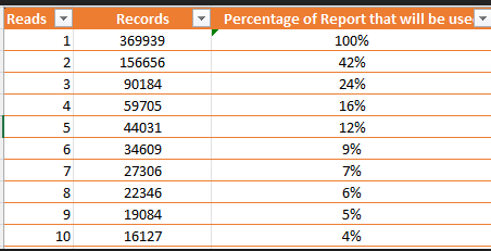
I have a great preference for percentiles because it transforms the VERY non-normal distribution of bacteria into a uniform distribution. One complicating factor with the common 16s tests is the number of reads required to deem a bacteria is there with a reliable measure. Many strains are single reads. If you require more reads, then the number of taxonomy items report drops quickly as shown in the table below.
To give a concrete example with real data, I am using the samples donated to my citizen science site that were processed through the UK based 16s provider, Biomesight.com. I am going to take a subset of those who entered self-reporting symptoms and divide them into two groups:
- Neurocognitive: Brain Fog issues reported (N:328)
- Neurocognitive: Brain Fog issues not reported (N:700)
The high number of Brain Fog is likely a byproduct of Long Covid in the population with those people willing to beat the bushes to find answers.
I am going to look only at genus level for illustration. A prior analysis found that species significance was more pronounced. I attached the data summary below. You can also download the data from Microbiome Prescription Citizen Science Data Repository and do your own data grinding. (Examine the data summary to determine the direction of shifts.)
| Probability | All | Reported | Prevalence | Percentile | Concurrent |
| < .01 | 68 | 20 | 5 | 42 | 0 |
| <.05 | 158 | 61 | 23 | 102 | 1 |
| < .10 | 241 | 102 | 36 | 147 | 0 |
Concurrent agreement between Significant Bacteria is quite dramatic as just one bacteria stands out: Oribacterium. If we exclude Prevalence, we find more.
- < .01
- Desulfosporosinus
- Blautia
- Sporolactobacillus
- Gallionella
- Paenisporosarcina
- Planococcus
- Limnobacter
- < .05
- Phascolarctobacterium
- Helicobacter
- Alkalihalobacillus
- Natronincola
- Alkaliphilus
- Oribacterium
- Cerasicoccus
- Salisaeta
- Anaerobranca
- Acetomicrobium
- Erysipelothrix
- Thioalkalivibrio
- Chryseobacterium
- Anaerotruncus
- Desulfurispora
- Lysinibacillus
- Halanaerobium
- Allochromatium
- Oleomonas
- Marinospirillum
- Moorella
- Agrococcus
- < .10
- Alishewanella
- Halomonas
- Ruminobacter
- Mobiluncus
- Leptothrix
- Dehalogenimonas
- Gemella
- Dorea
- Rikenella
- Brenneria
- Adlercreutzia
- Anaeroplasma
- Candidatus
- Endobugula
- Actinotignum
- Methylocella
- Ligilactobacillus
- Bergeyella
- Dickeya
Let us look at < .10 above, we have 641 genus, so .1 * 641 = 64 false positive would be expected. If you went down that path, you ignored that < .1 occurred over THREE measures. Assuming independence of each measure (for simplicity), then we have (0.1)3 or < 0.001; in other words, 0.001 * 641 = 0.6 false positive. Effectively, every genus listed above is statistically significant at < 0.001 for Neurocognitive: Brain Fog.
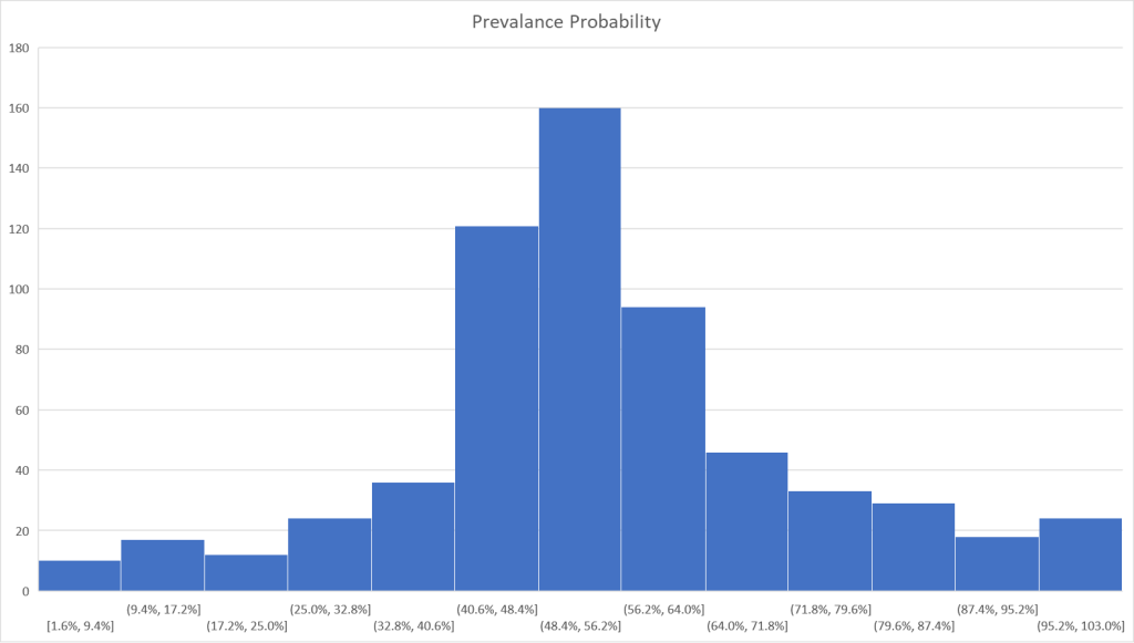
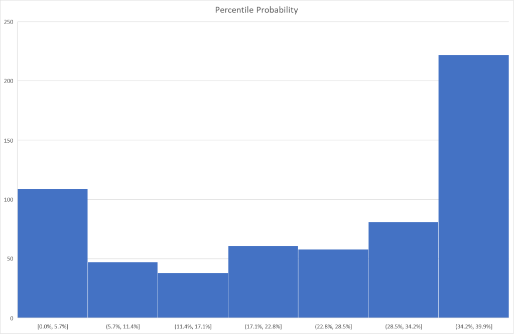
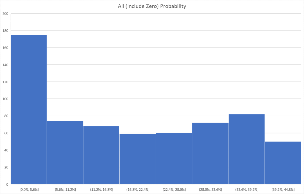
Some Visual Representations
I tend to use visuals to better understand processes. In this case, contrary to my expectations, we have quite dramatic differences in appearance. The first one looks like a normal distribution and the others definitely not normal distributions.

Bottom Line
The purpose of this post was to illustrate that no single method of determining significance is ideal. The use of prevalence is ideal for infrequently seen bacteria but is unlikely to produce results for commonly seen bacteria. It is important to understand the differences and ,in practice, do all five as a pro forma practice for microbiome data analysis.
The next question is simple, how do you treat people with brain fog? My own approach is to obtain a detailed microbiome sample (in this case, biomesight’s) and then identify which genus are sufficiently matching this pattern. From that matching, then use the fuzzy logic expert systems at Microbiome Prescription.com to suggest supplements, probiotics, diets and prescription drugs. There may be alternatice approaches to detemine a treatment approach.
Recent Comments