Ranged Odds Ratios is another phrase to described the concept of dose–response odds ratios that is classically seen with how cancer odds change as smoking exposure increases. Instead of number of cigarettes consumed, we use the amount of each taxa to indicate the risk of a symptom or disease.

With taxa, literature suggests that there is a range for each taxa. Studies using averages are likely a poor choice. More of a taxa is neither better nor worse for most taxa, rather whether it is in a range.

My database of volunteered microbiome samples, Microbiome Prescription, contains two broad categories of data:

• 16s samples: typically from biomesight, ombre, ubiome, etc
• Shotgun samples: typically from CosmosID, PrecisionBiome.eu, Thorne, XenoGene, Tiny Health

I developed the candidate ranged odds ratios for healthy (no symptoms or diagnosis) v unhealthy (has a symptom or diagnosis) by pooling these samples and using percentile ranking as an adjustment mechanism. The underlying assumption was that converting relative-abundance results to percentiles would compensate, at least partially, for differences in laboratory processing, sequencing approaches, and reporting pipelines.

This analysis tests that assumption: do the resulting odds ratios distinguish healthy from unhealthy samples equally well in 16S and shotgun data?

A secondary objective was to identify the taxonomic rank—species, genus, family, order, class, or phylum—at which the odds-ratio model performs best.

Method

A modified 90/10 train–test approach was used. For each test sample, I calculated the log odds ratio at each taxonomic rank. I then summarized results separately for healthy and unhealthy samples using both:

• The arithmetic mean of the log odds ratios.
• The median log odds ratio.
• Restricting to P < 0.01 or Chi square > 6.635

Results are shown in the tables below as:

$$\text{mean} \; / \; \text{median}$$

Using 16s Samples

For 16s samples, the genus level produced the strongest separation between healthy and unhealthy samples. A skew to the lower values is apparent from median < mean.

Tax Rank	Healthy	Unhealthy
Species	-27 / -24.7	-31.7 / -30.6
Genus	-36.8 / -32.9	-44 / -42.5
Family	-19.1 / -17.2	-22.8 / -21.5
Order	-8.3 / – 7.1	-10.6 / – 9.2
Class	-2.6 / -2.4	-3.1 / -2.8
Phylum	-4.7 / -4.7	-5 / -4.6
All (multiple counting via parent /child)	-97.3 / -84.2	-116.4 / – 115.8

At the genus level, the healthy versus unhealthy difference was approximately:

• 7.2 using the mean: $-36.8$−36.8 versus $-44.0$−44.0
• 9.6 using the median: $-32.9$−32.9 versus $-42.5$−42.5

This separation was substantially greater than at the other taxonomic ranks. Within this dataset and methodology, genus-level ranged odds ratios appear to be the most informative for 16S results.

Using Shotgun Samples

The shotgun results were unexpected. The model showed little or no ability to distinguish healthy from unhealthy samples, particularly at the species level, where I originally expected performance to be strongest.

Tax Rank	Healthy	Unhealthy
Species	-30.9 / -30.1	-30.9 / -30.1
Genus	-17.8 / -18.2	-16.7 / – 16.9
Family	-6.6 / -6.7	-6.2 / -6.3
Order	-1.9 / – 1.7	-2.1 / – 1.7
Class	0.2 / 0.8	0.2 / 0.8
Phylum	-1.8 / -1.5	-1.9 / -2

At the species level, the healthy and unhealthy values were identical: $-30.9 / -30.1$−30.9/−30.1 for both groups. Other ranks showed only small, inconsistent differences that would not provide a reliable basis for classification.

Refinement of P / Chi 2

Using 16s and taxa rank of genus, we will explore that the impact of different Chi Square values. Going to higher chi square values does not appear to do better separation of the categories.

Chi Square Threshold	Healthy	Unhealthy
3.84 (P < 0.05)	-36.8 / -32.9	-44 / -42.5
6.35 (P < 0.01)	-36.8 / -32.9	-44 / -42.5
10	-23 / -19.6	-27.3 / -26/1
20	-8.3 / -7.1	-10.2 / -8.9
40	-5.4/ -4.2	-6 / -4.2

Interpretation

One likely explanation is that the candidate ranged odds ratios were derived primarily from 16s data. Even after percentile normalization, the underlying taxa distributions may differ too much between 16s and shotgun pipelines for a shared model to work well.

This result also suggests that the difference between 16s and shotgun data may be more substantial than expected. Percentile ranking may reduce some cross-platform variation, but it does not necessarily make taxa measurements directly comparable across fundamentally different sequencing and bioinformatics workflows.

The poor shotgun performance could reflect one or more of the following:

• The training data were dominated by 16S samples.
• Species-level identification differs materially between 16S and shotgun methods.
• Taxonomic assignments, reference databases, filtering thresholds, and abundance calculations vary across reporting platforms.
• Percentile normalization does not adequately account for platform-specific measurement characteristics.
• There may be insufficient shotgun data to estimate stable ranged odds ratios.

Ranged Odds Ratios for specific symptoms or diagnosis is expected to perform much better. The definition of healthy and unhealthy lacks precision and is also self-declared.

Conclusions

The preferred approach is to develop ranged odds ratios using samples generated through the same processing flow as the samples to which the model will be applied. In practice, that means separate models may be needed for 16s and shotgun data—and potentially for individual laboratories or reporting pipelines.

The difficulty is obtaining enough comparable samples within each processing category to calculate stable odds-ratio ranges. Pooling data was a pragmatic attempt to test the methodology despite this limitation.

For the current dataset:

• Genus-level odds ratios performed best for 16s samples.
• The pooled model did not effectively distinguish healthy from unhealthy shotgun samples.
• Overall discrimination between healthy and unhealthy samples was modest rather than strong.
• Being symptom or diagnosis based is likely to produce better results.

The next step should be to build and validate separate 16s- and shotgun-specific odds-ratio models for explicit symptoms or diagnosis, then compare their performance using the same held-out test methodology.

Using the above 16s data, we can see that it appears to identify healthy individuals reasonably well.

Threshold	Healthy Percentage	Unhealthy Percentage
-32.4	74.4%	53.8%
-21	30.8%	22.3%
-42	87.2%	80.2%
-51	93.6%	93.8%

The key advantage of Ranged Odds Ratio is determining which taxa is the most probable contributor (highest chi square) and the likely contribution to the symptom or diagnosis (odds ratio).

Facebook Comment on this post:

I’m a nutritionist studying clinical nutrition. An ordinary nutritionist who has done certificate 4 in nutrition is not qualified on that level to assist people heal and build gut health. Once you start studying on the clinical level you get a very different training which now includes gut health thank goodness. I can tell you what foods to eat to build up your gut health see what to avoid but at the moment I’m not qualified to interpret test results. In fact I couldn’t really tell you who would be because doctors don’t study nutrition or food achieve or nutrition in a clinical level. Many dieticians who have been practicing for any length of time are quite behind in food science and gut health research because our knowledge is literally still being discovered. If you go the natural medicine route, they don’t do food science. Is it a case Ken of it’s anyone’s guess at the moment? The wellness industry is about profit through selling products not health.

The Hallucination Model

A clinician receives a microbiome report and see that 5 bacteria are outside of reference ranges according to the report. The clinician then searches the biomedical literature for an intervention on the US National Institute of Health that appears to move each of those taxa toward the report’s reference range and prescribes that intervention. This is prescribed to the patient. Mission accompanished.

Of course, any experienced clinician will know that he will not find such a study. A well-read clinician may be ROFL (Rolling on the Floor Laughing) with this approach for a variety of reasons:

• Reference ranges are typically done using means and standard deviation. This imposes an assumption of a normal distribution on the data. Microbiome data often exhibits a skew of 20-30; a skew over 2 excludes the use of a normal distribution. The term “normal” is often misunderstood; applying a casual conversation meaning instead of the statistical meaning. Laboratory reference intervals should not be confused with clinically meaningful targets. A reference interval is generally a statistical description of a selected comparison population, not evidence that a value outside that interval causes disease or that moving the value inward improves patient outcomes.
• It is extremely unusual for a clinical microbiome test to be the same as that used in any study. The National Institute of Standards and Technology has for over 10 years identified a severe lack of standardization as undermining microbiome research. Their lead has accurately stated in 2019: “There are currently 97 different ways to analyze the same raw data, and they will give you 97 different answers“. You cannot safely assume that the study results apply to the patient test.
• Finding all of the targeted bacteria in the same study is extremely unlikely. A common response is to find a study in isolation for each bacteria and then synthesize a combination of substances. This assumes complete independence of each substance and its bacteria influence. This is typically false with many substances helpful for one bacteria and contraindicated for another. To be safe, the clinician will need to read every published study for each substance; a time requirement impractical in a clinical setting.
• The impact of a substance on a bacteria may be inconsistent. Baseline microbiome composition and function, diet, lifestyle, antibiotic exposure, age, comorbid disease, and concomitant medications can all influence both microbial response and clinical effect. The direction of change observed in one population may not generalize to another, and a change in microbial abundance is not necessarily accompanied by an improvement in symptoms or disease outcomes.

A frustrated clinician (or patient) may simply asked some Large Language Model for an answer. The response would often be called hearsay in a court of law.

A fuller description is below.

Suggested Process

Ask the “expert” to read the above and explain how they work given this background paper. Expressions like “from experience” or “trust me” indicates a high risk of the person going to harm you instead of help you.

By Ken Lassesen, M.Sc.

Several years ago, I evaluated a broad range of statistical approaches for microbiome analysis, including machine-learning(ML) methods. I used publicly contributed samples available through the Microbiome Prescription citizen-science platform; the underlying dataset is available for download from its associated citizen-science repository.

At that time, I found that alternative statistical models generally outperformed the machine-learning approaches I tested. More recently, however, several direct-to-consumer microbiome testing companies have begun citing machine learning in their marketing materials. Time to revisit ML.

Perplexity summaries these as:

Company	What it claims about ML/AI
Viome	Says its tests use metatranscriptomics and ML models in its scoring engine; it states those models turn microbial and biochemical patterns into Viome Scores and dietary/supplement recommendations.
ZOE	Says it was founded to combine microbiome sequencing with ML, and that its PREDICT research data trained models underlying ZOE scores. Its retail gut test uses shotgun metagenomics, though its ML claims also cover its broader personalized-nutrition predictions rather than only the stool-test report.
BIOHM Health	Markets the Longevity Gut Score as using “advanced AI,” and trade reporting attributes its aging-related model to machine- and deep-learning methods trained on more than 10 million data points,
FeelGut	Claims its sequencing reads are processed through a “machine learning bioinformatics pipeline,” compared with reference libraries and its own data set to produce health scores and food suggestions
EZBiome	Says it applied ML and AI to a database of more than 120,000 people to generate a global microbiome health index.
Tiny Health	Tiny Health says it uses machine learning with an individual’s sequencing results and survey data to personalize its diet, supplement, and lifestyle recommendations.

Perplexity also informs me that none have “not publish enough to reproduce its proprietary scoring and recommendations.” Thus the question must be asked, is this marketing hype or validated peer-reviewed science.

Looking at some of the literature

Microbiome ML results can look better than they generalize because the data are sparse, compositional, high-dimensional, and highly affected by batch effects. Differences in DNA extraction, sequencing platform, 16S variable region, taxonomic database, geography, diet, medication exposure, and disease-site recruitment can all be learned by a model instead of the biological signal of interest.

Extract from Machine learning approaches in microbiome research: challenges and best practices [2023]

Which further stated

Microbiome data is often high-dimensional, with more features (microbial genes or taxa) than samples. This can lead to overfitting and poor generalization, especially with small sample sizes. Feature filtering and selection methods are employed to reduce dimensionality, but different methods can yield different results, and correlated features can hinder selection.

The different results from using different methods is a major red flag🚩 for me.

The substantial variability in results produced by different analytical methods is a significant concern. In colloquial terms, there is a risk that artificial-intelligence systems may generate plausible but poorly supported inferences, while analysts may—intentionally or unintentionally—select modeling choices that align with organizational expectations. Highly favorable results can sometimes be obtained through extensive tuning, but the central methodological question remains: do the findings reflect genuine signal in the data, or artifacts introduced through model selection and optimization?

To examine this issue, I conducted a preliminary evaluation of relatively naïve machine-learning models across several collections of microbiome samples, including samples originating from BiomeSight, uBiome, and Ombre. Here, “naïve” refers to simple, out-of-the-box implementations using Microsoft.ML.Data and publicly downloadable data, without extensive feature engineering, hyperparameter optimization, or other model-tuning procedures.

The Core Code in C#

var classifier = new VariableLengthBinaryClassifier();
var data = DataDal.ML_Symptoms(source, sympid);//Array of {condition, double[] }
IReadOnlyList reports =
classifier.Train(data);
var result = classifier.Predict(data[0].Values);
var line = $"{source},{name},Accuracy={reports[0].Accuracy}; ";

I evaluated two representations of taxonomic abundance:

• Relative abundance expressed as percentages.
• Quintile-based categories:
  • Not detected
  • Detected through the 25th percentile
  • 25th–50th percentile
  • 50th–75th percentile
  • Above the 75th percentile

My preregistered practical criterion was straightforward: model accuracy should exceed 0.50. Because a binary classifier can achieve approximately 0.50 accuracy through random prediction under balanced classes, results below this threshold would provide little evidence of useful predictive performance. Across several hundred tested scenarios, the full quintile taxonomic model has associations between 0.429 and 0.447 over 1919 dimensions . Detailed results are provided in the appendix.

Interpretation of the findings

These results require careful qualification. More favorable predictive performance may be achievable when analyses are tightly controlled for population characteristics, sequencing methodology, bioinformatic processing, and other sources of technical and biological variation. However, models developed under such restrictive conditions may generalize only to highly similar populations and to data processed through the same microbiome-analysis pipeline. This limitation is particularly important given the substantial effects that laboratory methods, reference databases, taxonomic classification procedures, and other pipeline choices can have on microbiome results.

The samples used in this evaluation were comparatively heterogeneous: they were uploaded by individuals from diverse locations and backgrounds, although samples within a given retail-laboratory source were processed using the same general pipeline. For potential clinical application, such “real-world” heterogeneity is important, because clinical tools must ultimately perform outside narrowly selected research cohorts. Any published findings should therefore not be interpreted as universal evidence from machine learning in microbiome research; rather, they indicate limited suggestions for the specific datasets, prediction tasks.

Impact of restricting to a Taxonomy Rank

A follow up exploration using quintile-based categories filtered to specific taxonomy ranks resulted in the following accuracy.

• Phylum: 0.73 over 31 dimensions
• Class: 0.73 over 61 dimensions
• Order: 0.73 over 123 dimensions
• Family: 0.64 over 268 dimensions
• Genus: 0.52 over 524 dimensions
• Species: 0.46 over 795 dimensions

In general, as the number of vectors (taxonomies) increases, the reported accuracy decrease.

Metabolite-based analysis

In earlier work, I found that estimated metabolite profiles were more useful symptom predictors than taxonomic abundance alone. These metabolite estimates were derived using functional inferences based on the Kyoto Encyclopedia of Genes and Genomes (KEGG).

A subsequent analysis using metabolite-based features produced substantially better results. In most scenarios, accuracy exceeded 0.50, and the highest observed accuracy was 0.609. This suggests that inferred functional or metabolic characteristics may contain more clinically relevant predictive information than taxonomic composition alone, at least for the outcomes examined.

Over 2293 dimensions, accuracy ranged from 0.56 to 0.618, a much larger spread then above.

Clinical implications

This produces an important practical dilemma:

Feature type	Primary advantage	Primary limitation
Taxonomic profiles	A large literature describes interventions, dietary factors, and substances associated with changes in particular taxa	Taxonomy showed limited predictive performance in these minimally tuned models
Estimated metabolites	Better predictive performance in this analysis	Comparatively limited evidence identifies interventions that reliably modify specific inferred metabolites

At present, I therefore prefer alternative statistical models and taxonomic features for generating practical suggestions, largely because the supporting intervention literature is more extensive. Although retail microbiome-testing companies may indeed use machine-learning methods, I remain cautious about the predictive accuracy and clinical utility achieved by their proprietary models. Claims of machine-learning capability may be commercially attractive, but the relevant question is whether these approaches produce reproducible, clinically meaningful improvements for clients. Peer-reviewed evidence demonstrating such benefit remains the standard needed to support those claims.

At this time of writing, there were 555 users in the last year uploaded to the Microbiome Prescription citizen-science platform. 326 of these users have done two or more uploads in the same year or a 59% repeat rate. This suggests that the suggestions provided were sufficiently beneficial that about 60% of users did a repeat test to get new suggestions.

Postscript: My Preferred Approach

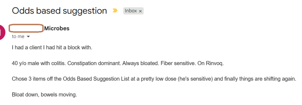
It is an old classic, Ranged Odds-Ratios. In published literature, you will find the odds of getting lung cancer ranged against the number of cigarettes smoked daily. A morning email shows that it can work for seasoned medical professionals who have tried all of the usual approaches without success. I have seen it dropped a hypertension person drop their systolic blood pressure by 30 mmHg in just over a week.

The typical pipeline processing finds the closest match of 16s or shotgun to a reference library. Conceptually this is fine, but when the closest match is not a bacteria found in humans (or very rarely), then the match may have zero value. It is speculative information for information sake.

Some examples from the taxon reported in retail microbiome reports:

• Sharpea azabuensis:  isolated from the faeces of thoroughbred horses in 2008
• Olsenella timonensis:isolated in 2015
• Phoenicibacter congonensis: isolated in 2019 from a Pygmy
• Gillisia: From marine environment
• Macrococcus: Found in food animals
• Clostridium chauvoei:  causative agent of blackleg, a wide spread serious infection of cattle and sheep with high mortality

At the very least, the matching should be done to those reported in humans.

This creates a challenge for the clinician — there is no literature on these bacteria.

But to the capable statistician…

They can often be very useful for determining odds ratios for a specific condition or general good health. A suitably large dataset is needed (thousand of samples). This leaves the clinician between the rock (no literature or studies) and a hard place (“magical” statistical odds ratios).

Recently, I released Odds Ratio–based suggestions and reports, such as the example shown here.

The underlying concepts are straightforward:

• If you are in an unhealthy range, the goal is to move out of that range.
• If you are not in an unhealthy range but fall outside a defined healthy range, the goal is to move into the healthy range.

For healthy ranges, interpretation is simple—you are either too high or too low, so the direction of adjustment is clear.

• If the range is 10%ile to 30 %ile and you are at 29%ile, should you increase or decrease?
• If the range is 70%ile to 90 %ile and you are at 85%ile, should you increase or decrease?

Unhealthy ranges, however, are more nuanced.

For example:

• If the unhealthy range is the 10th to 30th percentile and your value is at the 29th percentile, should you increase or decrease?
• If the unhealthy range is the 70th to 90th percentile and your value is at the 85th percentile, should you increase or decrease?

The core issue is understanding why the range is considered unhealthy—specifically, whether the problem arises from having too little of something or too much.

• Lactobacillus delbrueckii
  • Unhealthy: 0 – 45%ile
  • Healthy: 48%- 72%ile
• Lactobacillus gasseri (A Surprise!): 0 -100%ile is Unhealthy
• Lactobacillus johnsonii: 0 – 72%ile Healthy
• Lactobacillus taiwanensis: 23-56%ile Unhealthy
• Limosilactobacillus reuteri: 0-52%ile Unhealthy

The above numbers are slightly suspect because many are P > 0.002, so may not be significant.

Confidence	Bacteria this or less significant	Bacteria More Significant
P < 0.001	2081 Ranges	694 Ranges
P < 0.0001	2383 Ranges	392 Ranges
P < 0.00001	2495	280

A List of Families with high significance

It is interesting to note that neither Lactobacillaceae (Lactobacillus) nor Bifidobacteriaceae (Bifidobacterium) were found to be significant at this level. Nor were they at the genus level, only at the specific species level (see below)

tax_name	Range	Nature
Anaplasmataceae	0 to 75	Unhealthy
Bartonellaceae	0 to 79	Unhealthy
Chlorobiaceae	0 to 58	Unhealthy
Chrysiogenaceae	0 to 83	Unhealthy
Clostridiales Family XVI. Incertae Sedis	0 to 100	Unhealthy
Comamonadaceae	0 to 28	Unhealthy
Comamonadaceae	34 to 52	Unhealthy
Cyanobacteriaceae	21 to 99	Unhealthy
Deinococcaceae	0 to 46	Unhealthy
Desulfonatronaceae	0 to 50	Unhealthy
Enterococcaceae	0 to 66	Healthy
Enterococcaceae	68 to 71	Unhealthy
Euzebyaceae	13 to 100	Unhealthy
Hyphomicrobiaceae	0 to 87	Unhealthy
Kiloniellaceae	20 to 99	Unhealthy
Legionellaceae	0 to 100	Unhealthy
Listeriaceae	74 to 88	Unhealthy
Litorivicinaceae	0 to 18	Unhealthy
Lysobacteraceae	0 to 27	Unhealthy
Methylophilaceae	0 to 96	Unhealthy
Nostocaceae	14 to 88	Unhealthy
Oxalobacteraceae	0 to 30	Unhealthy
Pseudanabaenaceae	0 to 100	Unhealthy
Shewanellaceae	0 to 73	Unhealthy
Sporolactobacillaceae	0 to 100	Unhealthy
Streptosporangiaceae	53 to 88	Unhealthy
Symbiobacteriaceae	0 to 81	Unhealthy
Synechococcaceae	0 to 9	Unhealthy
Synechococcaceae	48 to 85	Unhealthy
Thermoanaerobacterales Family III. Incertae Sedis	3 to 50	Unhealthy
Thiotrichaceae	7 to 100	Unhealthy
Weeksellaceae	0 to 100	Unhealthy

Significant Bifidobacterium Species

tax_name	Range	Nature
Bifidobacterium adolescentis	0 to 49	Unhealthy
Bifidobacterium angulatum	0 to 73	Healthy
Bifidobacterium breve	0 to 76	Unhealthy
Bifidobacterium catenulatum	0 to 100	Healthy
Bifidobacterium dentium	0 to 50	Unhealthy
Bifidobacterium scardovii	0 to 79	Unhealthy

Significant Lactobacillus Species

tax_name	Range	Nature
Lacticaseibacillus brantae	33 to 70	Unhealthy
Lactobacillus acidophilus	0 to 76	Unhealthy
Lactobacillus amylovorus	0 to 100	Unhealthy
Ligilactobacillus murinus	0 to 100	Unhealthy

Summary

I am hoping to expand the size of my “Healthy Samples” in the next weeks. This should improve the ranges and significance.

An early user of the Odd Ratio approach (see New Suggestions Approach and Ranges for Healthy and Unhealthy Bacteria) raised concerns about some of the bacteria identified.

For example, Odoribacter denticanis was only 0.002%, Clostridium akagii was 0.002%, and Symbiobacterium was 0.004%. The natural question is whether bacteria present at such tiny levels could have any meaningful impact. Interestingly, these values are not extreme outliers; they appear to be fairly common at these levels.

There are several ways to approach microbiome adjustment. One is to focus on bacteria that dominate the microbiome. Another is to target bacteria with extreme values. A third is to focus on bacteria whose mechanisms of impact are known, such as those that produce metabolites linked to leaky gut.

My own approach is based on strong statistical associations. Association does not prove causation, and in microbiome research, the causal details are often not well established. My working assumption is that bacteria strongly associated with a condition are likely influencing it, perhaps through metabolites they produce or consume. If so, reducing those bacteria should reduce the metabolic effect.

The low-abundance dilemma

The microbiome can be thought of as a population, much like a country’s human population. If there were 989 billionaires[Forbes] in the United States, that would still be only about 0.0003% of the population. Yet few people would conclude from that alone that billionaires have little influence on the country. In practice, a very small number of highly influential actors can still shape outcomes in major ways.

The same logic applies to microbiome analysis. Low abundance does not necessarily mean low impact.

The odds ratios used here are not based on an ideal dataset, but on the best data currently available. The choice is not between perfect evidence and flawed evidence; it is between using the best evidence now or waiting indefinitely for perfect data. In that sense, this is a best-effort approach grounded in the data we have rather than silence in the face of incomplete evidence.

Reader Response

I think the question is whether such low values represent an actual organism or noise. I remember in the days of Ubiome, a reading of 0.001% meant only a single organism was found. Ubiome actually discarded it if there was only one found. They only reported if there were two or more. Thryve otoh, reported everything, which is one of the reasons they found more than Ubiome.

ofc, some of these results are more than one organism, but the question still remains as to whether this is a real organism or noise. It just seems that there are a lot of variables in this analysis with big error margins, and you are compounding them by bundling them all together. The error margin in the final result is likely huge.

Resolution

The way to handle this issue was requiring the raw count to be at least 5. This should reduce the noise level to acceptable levels. The dilemma remains on identification differences between tests (See this post for details). With aggregation across different tests, this issue should be reduced.

In the decades that I have been working with the microbiome, the scientist in me have become very troubled. Some of the key concerns have been:

• Massive inconsistency between tests results in terms of percentage of different bacteria found [more information]
• Medical practitioner picking certain key bacteria to focus on based on rote or hearsay.
  • No studies showing any bacteria are more important than other possible bacteria.
• Suggestions often do not consider counter-indication / adverse effects on other bacteria
• Healthy ranges are determined using normal distributions (Normal Range) which is grossly invalid given the typical bacteria distributions [more information]

Microbiome Prescription current suggestion algorithms appears to have over a 75% chance of improving microbiome tests results (with typical subjective improvement reported) [more information]. For those not responding well to those suggestions, I have been researching an alternative, more rigorous, approach based on computationally intense computation. This method is not practical to run on a website, instead it is computed off-line and then emailed to the person.

The new suggestions are based on the following:

• Using Percentile ranking for better comparison
• Using Odds Ratios (a rigorous statistical process using P < 0.001) to select bacteria
• Every suggestion is checked against every selected bacteria to insure no adverse effect

For more details see “A Proposed Model for Clinical Use of the Human Microbiome“

The new suggestions set consists of three reports:

• Focus on the top 20 bacteria associated with being unhealthy
• Focus on the top 20 bacteria associated with being healthy
• Focus on the top 40 bacteria associated with both unhealthy and healthy

Selection is based on the statistical significance. Why three? As more and more bacteria are added to the target bacteria, the fewer modifiers are left that does not have adverse effect on some of the bacteria.

A knowledgeable reader raised some very valid questions here: Questions about using Odds Ratio

Example Reports:

Unhealthy Bacteria

The goal is to shift the bacteria outside of the unhealthy range. Often it is to eliminate it, but in other cases it may be just to push it up and outside the range.

1. Nostocaceae [family] [1162] 47.5 %ile Unhealthy Range [14 – 88], Plan:Decrease
   Signif: 36.74, Odds:-4.34
   Decreases This Bacteria
   • No Substances without adverse effect on other bacteria
2. Klebsiella [genus] [570] 46.1%ile Healthy Range [1 – 56], Plan:Increase
   Signif: 26.39, Odds:-3.40
   Increases This Bacteria
   • 4 :non-starch polysaccharides @Sugar and similar
   • 2 :Catechol {Catecholamines} @Flavonoids, Polyphenols etc
   • 2 :Escherichia coli:DSM 16441-16448 {symbioflor-2} @Probiotics
   • 2 :Ceratonia siliqua {carob} @Food (excluding seasonings)
   • 2 :115 different soil based taxa {General Biotics Equilibrium} @Probiotics
   • 2 :Laurencia tristicha {Marine red algae} @Food (excluding seasonings)
   • 2 :L-3-hydroxytrimethylaminobutanoate {carnitine} @Amino Acid and similar

Healthy Bacteria

The goal is to shift into the optimal range

1. Enterococcaceae [family] [81852] 87.2%ile Healthy Range [1 – 66], Plan:Decrease to Healthy Range
   Signif: 20.57, Odds:0.97
   Decreases This Bacteria
   • 7 :Shen Ling Bai Zhu San {参苓白术散} @Herb or Spice
   • 6 :Sambucus nigra L. ssp. canadensis {Elderberry} @Food (excluding seasonings)
   • 5 :Chamaemelum nobile {Camomile} @Herb or Spice
   • 5 :Olea europaea {Olive leaf} @Herb or Spice
   • 5 :Ocimum tenuiflorum {Tulsi} @Herb or Spice
   • 5 :Micromeria fruticosa {White-leaved Savory} @Herb or Spice
   • 5 :Eucalyptus {Gum Tree} @Food (excluding seasonings)
   • 5 :Arctostaphylos uva-ursi {Bearberry} @Food (excluding seasonings)
   • 4 :helichrysum italicum {Immortelle} @Herb or Spice
   • 4 :Dysphania ambrosioides {Epazote} @Food (excluding seasonings)
   • 4 :Sinapis alba {yellow mustard} @Food (excluding seasonings)
   • 4 :Cathelicidin antimicrobial peptide {LL37} @Amino Acid and similar
   • 3 :Bixa orellana {annatto } @Herb or Spice
   • 3 :Rhus coriaria {Sumac} @Herb or Spice
   • 2 :Withania somnifera {Ashwagandha} @Herb or Spice
2. Streptococcus alactolyticus [species] [29389] 99.0%ile Healthy Range [1 – 75], Plan:Decrease to Healthy Range
   Signif: 17.33, Odds:1.55
   Decreases This Bacteria
   • 5 :Olea europaea {Olive leaf} @Herb or Spice
   • 5 :Micromeria fruticosa {White-leaved Savory} @Herb or Spice
   • 5 :Eucalyptus {Gum Tree} @Food (excluding seasonings)
   • 5 :Sodium Bicarbonate {Baking Soda} @Common and OTC Supplements
   • 5 :Prunus mume {Umeboshi} @Food (excluding seasonings)
   • 4 :helichrysum italicum {Immortelle} @Herb or Spice
   • 4 :chlorhexidine @Common and OTC Supplements
   • 3 :Bixa orellana {annatto } @Herb or Spice
   • 3 :Rhus coriaria {Sumac} @Herb or Spice
   • 2 :Withania somnifera {Ashwagandha} @Herb or Spice
   • 2 :Bifidobacterium longum subsp. longum BB536 {BB536} @Probiotics
   • 2 :Xylaria hypoxylon {candlesnuff fungus} @Food (excluding seasonings)

Both Healthy and Unhealthy

Because the number of bacteria increases, the number of modifiers decrease,

1. Nostocaceae [family] [1162] 47.5 %ile Unhealthy Range [14 – 88], Plan:Decrease
   Signif: 36.74, Odds:-4.34
   Decreases This Bacteria
   • No Substances without adverse effect on other bacteria
2. Klebsiella [genus] [570] 46.1%ile Healthy Range [1 – 56], Plan:Increase
   Signif: 26.39, Odds:-3.40
   Increases This Bacteria
   • 4 :Catechol {Catecholamines} @Flavonoids, Polyphenols etc
   • 3 :Escherichia coli:DSM 16441-16448 {symbioflor-2} @Probiotics
   • 3 :L-3-hydroxytrimethylaminobutanoate {carnitine} @Amino Acid and similar
3. Acidaminococcus [genus] [904] 55.2%ile Healthy Range [21 – 65], Plan:Increase
   Signif: 23.71, Odds:-3.42
   Increases This Bacteria
   • No Substances without adverse effect on other bacteria
4. Thiotrichaceae [family] [135617] 19.6%ile Unhealthy Range [7 – 100], Plan:Decrease
   Signif: 23.27, Odds:-3.42
   Decreases This Bacteria
   • No Substances without adverse effect on other bacteria
5. Oscillospira guilliermondii [species] [119853] 67.1%ile Healthy Range [2 – 71], Plan:Increase
   Signif: 22.46, Odds:-3.37
   Increases This Bacteria
   • No Substances without adverse effect on other bacteria
6. Fusobacterium [genus] [848] 43.3%ile Healthy Range [1 – 70], Plan:Increase
   Signif: 20.81, Odds:-1.67
   Increases This Bacteria
   • 6 :Citricidal {Grapefruit seed extract} @Food (excluding seasonings)
   • 2 :pediococcus acidilactici {P acidilactici} @Probiotics

The Avoid List

This lists the items with the number of bacteria it may adversely impact.

Counter Indicated Modifiers

• 18 :Slow digestible carbohydrates. {Low Glycemic} @Diet Style
• 16 :Bovine Milk Products {Dairy} @Food (excluding seasonings)
• 15 :bacillus @Probiotics
• 15 :whole-grain diet @Diet Style
• 15 :bacillus,lactobacillus,streptococcus,saccharomyces probiotic @Probiotics
• 14 :Hordeum vulgare {Barley} @Food (excluding seasonings)
• 14 :dietary fiber @Diet Style
• 14 :High-fibre diet {Whole food diet} @Diet Style
• 14 :Lacticaseibacillus paracasei {L.paracasei} @Probiotics
• 14 :Limosilactobacillus reuteri {L. Reuteri} @Probiotics
• 14 :wheat @Food (excluding seasonings)
• 14 :yogurt @Food (excluding seasonings)
• 14 :Fiber, total dietary @Diet Style
• 13 :bacillus subtilis {B.Subtilis } @Probiotics

How do you get these Reports?

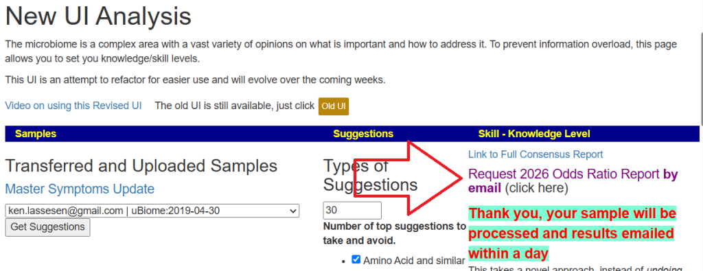
When new suitable samples are uploaded, these reports are automatically generated and email within a day.

If you want an older sample processed, just click this link on the site

Note: If you do not receive it in 36 hours, check your spam and trash folders.

After some user feedback, a single report is sent. This report looks at bacteria in the unhealthy range and those that are outside of the healthy range. Most bacteria has one OR the other.

DIRECT LINK TO TABLE

In common medical practice, bacteria ranges tend to be very random. Often it becomes values above or below average plus/minus 1.96 Standard Deviations. Bacteria are abnormal (i.e. are not a normal or bell curve distribution).

My training is in statistics and operations research. This post and other posts are intended to ask “why not do things this way” and to inspire lifting the bar in approaching the microbiome.

From some 7,500 samples I computed statistical ranges for 2,470 different bacteria with a threshold of Chi² > 6.6 (around p < 0.01). The higher the odds, the more significant. The ranges apply only is the bacteria was detected in the sample. The page is available here.

Some Highlights

• Lactobacillus is unhealthy if below the 68%ile
• Bifidobacterium is unhealthy if below the 16%ile
• Akkermansia muciniphila is unhealthy if below the 36%ile

Some bacteria appear to have no ranges, for example: Bacteroides, Firmicutes  

Example of one bacteria with multiple ranges

• Blautia producta
  • Below 19%ile Unhealthy
  • 20 -26%ile Healthy
  • 27 -38%ile Unhealthy
  • Over 38%ile no statistically significant impact
• Bifidobacterium bifidum
  • Below 25%ile Unhealthy
  • 26 -28%ile Healthy
  • 32 -42%ile Unhealthy
  • Other values – no statistically significant impact
• Bifidobacterium dentium
  • Below 50%ile Unhealthy
  • 51 -64%ile Healthy
  • 65 -73%ile Unhealthy
  • Other values – no statistically significant impact
• Rickettsiales
  • 0 – 100% is unhealthy!

Summary

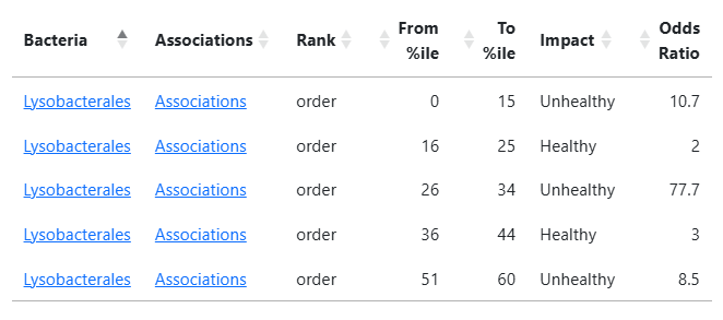
So far, most of the numbers appear to follow common sense (see Highlights above). Bacteria with multiple ranges is more of a challenge to understand and exposes a concept close to a “Yin/Yang” of the microbiome.

A more interesting one is: Lysobacterales. The low odds ratios for healthy hints that we may wish to discard those values resulting in < 60 as unhealthy.

Adding to Microbiome Prescription

I am planning to add it as a bacteria selection method using a higher Chi² value then used for the demo table. Stay tune.

I will be using P < 0.001 to safely identify the bacteria of concern.

The organization Vitract.com recently referenced Jona Health during a conference call, noting that Jona’s platform reportedly incorporates approximately 200,000 studies. This claim prompted closer examination, particularly regarding how such figures are defined and communicated.

Public-facing descriptions of Jona’s methodology indicate that its system has “read” approximately 220,000 peer-reviewed studies, with an ongoing ingestion rate of roughly 2,000 new studies per month as microbiome research evolves. However, the distinction between studies that are “read” versus those that are critically evaluated and actively utilized is nontrivial. The use of the term “read” appears to function as a marketing construct, potentially conflating exposure to literature with meaningful incorporation into a validated analytical framework.

For comparative purposes, equivalent metrics from the Microbiome Prescription database demonstrate substantially greater scale and curation rigor. The system has processed a total of 2,953,169 studies—an order of magnitude greater than the figures cited above. Recent weekly ingestion rates further illustrate this difference:

• May 29, 2026: 5,871 new studies
• May 22, 2026: 4,984 new studies
• May 15, 2026: 5,584 new studies
• May 8, 2026: 5,582 new studies

Importantly, each study undergoes manual review prior to inclusion, reflecting the inherent complexity and nuance of microbiome literature that cannot be reliably interpreted through automated methods alone.

More critical than raw ingestion counts is the subset of studies that yield actionable, high-quality data. Within the Microbiome Prescription system, 21,391 studies have been identified as containing usable information and are actively incorporated into the knowledge base. These curated studies underpin approximately 14,518,553 PubMed-derived data points within the expert system. In addition, the platform includes approximately 71,000 experimentally derived bacterial interaction data points sourced from raw datasets.

These distinctions underscore the importance of evaluating not only the quantity of literature processed but also the depth of curation and the proportion of data that is methodologically sound and practically usable.

In conclusion, numerical claims regarding literature scale should be interpreted with caution, particularly when used in marketing contexts. The critical question is not how many studies are nominally “read,” but rather how many are rigorously evaluated and meaningfully integrated into a reliable analytical framework. Microbiome Prescription operates as a not-for-profit, citizen science initiative with the explicit goal of advancing microbiome-informed decision-making through careful curation and transparent methodology, rather than promotional positioning.

Bottom Line

As with all things marketing “Where’s the beef?” and not the hype. Microbiome Prescription is a not profit seeking citizen science endeavor seeking to improve the use of the microbiome.

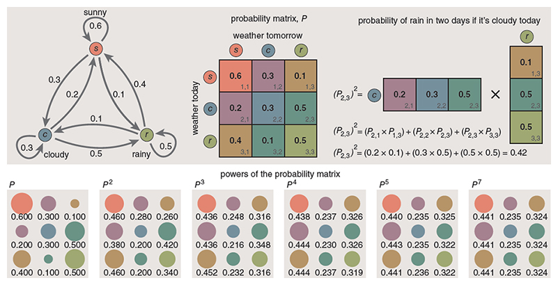
During my Probability and Statistics studies in the early 1970s, I developed a strong interest in Markov chains. The core idea behind a Markov process is straightforward: the next state of a system depends only on its current state and a set of transition probabilities. Given that the microbiome is full of interactions, it seems the ideal model.

In practical terms, this can be represented as a matrix—similar to an Excel spreadsheet—where each column represents an intervention or event, and each row represents a state variable. When a given event occurs, its associated column of values describes how each variable is expected to shift.

To illustrate this concept in a microbiome context, consider a simplified model using R²-derived relationships between probiotics and bacterial taxa. In this matrix, each value represents the directional influence of a probiotic on a specific bacterium, where zero indicates no measurable effect.

Example interaction matrix:

Target Bacteria	Pro 1	Pro 2	Pro 3	Pro 4
A	-0.23	0.44	0.11	0.00
B	0.2	0.32	-0.22	0.14
C	0.18	-0.11	0.11	0.12
D	-0.31	0.13	0.22	-0.28

From this, we can evaluate each probiotic independently by applying its column to the current microbiome state and observing whether each bacterium moves toward or away from its target range.

A simplified qualitative interpretation might look like this:

Target Bacteria	Pro 1	Pro 2	Pro 3	Pro 4
A	n/a	worse	worse	need improvement
B	worse	worse	better	worse
C	n/a	worse	better	better
D	n/a	worse	worse	better

In this example, Probiotic 1 appears to be the best initial choice, as it minimizes negative outcomes relative to the others.

Once the first intervention is applied, we update the microbiome to its predicted new state. This updated state becomes the input for the next evaluation cycle. For instance, after adjusting bacterium B, we might find:

Target Bacteria	Pro 1	Pro 2	Pro 3	Pro 4
B	worse	worse	better	n/a

This suggests that Probiotic 3 is the most suitable follow-up intervention for B.

In practice, this process must be applied across all bacteria simultaneously—including those currently within the acceptable range—to generate a full predicted microbiome after each intervention. The goal is to evaluate all candidate substances and select the one that produces the greatest overall improvement.

By iterating this process, we can construct a sequence of interventions such as:

• Herb 1
• Probiotic 2
• Diet Change 3

Once a candidate sequence is identified, it is important to test whether the order of interventions materially affects the outcome. This can be done by randomizing the sequence and comparing predicted results. If the sequence proves immaterial, then some interventions may be applied concurrently rather than sequentially.

That is the basic concept, the mathematics are a little more complex. How do you estimate the amount of shift?

A Rule of Thumb

My working assumptions are:

• All bacterial abundances are converted to percentiles, with defined target percentile ranges.
• For probiotics, assume a ±10 percentile shift scaled by the R² relationship for a given bacterium.
• For other substances, estimate impact based on available studies:
  • One study: approximately 1 percentile shift.
  • Mixed evidence: net effect equals positive studies minus negative studies (e.g., 8 positive and 2 negative yields a 6 percentile shift).
  • Cap the maximum effect at 10 percentiles regardless of study volume.

These values are approximations and likely imperfect, but they provide a consistent framework given current data limitations.

Method Summary

1. Convert microbiome measurements into percentiles.
2. Identify bacteria that fall outside their target ranges.
3. Apply each candidate intervention to the current state and compute the predicted microbiome.
4. Select the intervention that produces the greatest reduction in out-of-range bacteria (or other chosen objective function).
5. Update the microbiome to this predicted state.
6. Repeat the process until all bacteria are within range or no further improvement can be achieved.

The result is an ordered sequence of interventions designed to progressively normalize the microbiome. Questions of dosage, duration, and clinical appropriateness are intentionally excluded from this model and should be addressed by qualified professionals.

This is a major transition from “Let us try this and see what happens” to an objective/numeric prioritization based on a reasonable mathematic model. Odds are, that the results will be better for the patient.