In this post I will show the results of a series of experiments using the results of prior posts, . The philosophical question being asked is this “How useful is a result showing that genus X mean is higher with a condition then without for screening individuals?” (i.e. with statistical significance of P < 0.01 or better).

Often studies will provide a statement such as the one shown below.

Men with higher VFA harbored a smaller relative abundance of Blautia and Bifidobacterium (P for trend: 0.003 and 0.021, respectively),

Blautia genus associated with visceral fat accumulation in adults 20-76 years of age [2019]

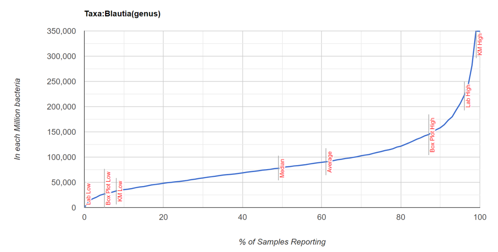
While it is possible to compute the t-score from p < 0.003 [assuming sample size of 100 was used, then 2.871] and then a priori apply it to the mean and standard deviation of population for a specific lab (per million) [mean: 89,844, standard deviation: 60,542] and get a proxy mean for male VFA = mean – 2.871 * StdDev/ 10 => 43,160.

We do not have an answer for the probability of a sample with 50,000 or 20,000 units. We could assume we have a normal distribution but that is an naïve assumption. A normal distribution would have average and median co-located. For some bacteria, the mean is at the 90th percentile.

On my citizen science site, I kludged in some prediction algorithms which has been well received (including by medical practitioners reporting that it often identifies symptoms that the patient forgot to mention). I would like to improve and validate these prediction algorithms using more traditional methods.

This is a bit of a wandering post as I explore various approaches.

To investigate this, I am using a dataset processed through a single process (Biomesight.com) of 2585 samples (the Population). From these 2585 samples, we compute the percentile ranking of the percentage of each taxa. Of these samples, some 1080 (the Sample) have annotated with self-declared symptoms or conditions with 279 different symptoms. We selected only symptoms with more than 36 samples annotated with that symptom. We will work at the genus level only so each variable is conceptually reasonably independent.

With this data, we will try to construct and then test models for the hundred of symptoms sets available.

Foundations

We start with the t-scores we obtained from regression on the count per million of each genus against symptoms [1 below]. There are multiple of other possibilities as shown below. These were initially explored and none showed significant better results than [1] after running 48,000 models.

1. Based on the average, standard deviation, ratio between with and without symptom of the percentage of the microbiome — ignoring not reported [C]
2. Based on the average, standard deviation, ratio between with and without symptom of the percentage of the microbiome deeming not reported to be a zero [CN]
3. Based on the average, standard deviation, ratio between with and without symptom of the percentile over all samples — ignoring not reported [P]
4. Based on the average , standard deviation, ratio between with and without symptom of the percentile over all samples — deeming not reported to be a zero [PN]
5. Based on those above or below the Nth percentile between with and without symptom — ignoring not reported [#]
6. Based on those above or below the Nth percentile between with and without symptom — deeming not reported to be a zero [#N]

Percentiles can be useful because it transforms the data into a uniform continuous distribution and should always be explored with microbiome data. I will return to this in subsequent posts.

T-scores

Each genus to symptom analysis results in a t-score. We will use the following 4 values in our tests.

• 1.28 (90%)
• 2.33 (99%)
• 3.10 (99.9%)
• 3.73 (99.99%)

In our regression analysis we obtain the following average counts across symptoms. We also factor in prevalence since some significant genus may be rarely seen to determine the expected number of genus that a sample may have reported that matches our regression pattern.

• t-score: 1.28: average number of genus: 317, with prevalence factored in: 94
• t-score: 2.22: average number of genus: 294, with prevalence factored in: 85
• t-score: 3.1: average number of genus: 270, with prevalence factored in: 76
• t-score: 3.73: average number of genus: 243, with prevalence factored in: 64

Number of Standard Deviations

The process of doing +/- 1 standard deviation will eliminate some significant genus, if the value is below zero or above the population (a nominal 1,000,000) the using it as a test becomes moot.

• t-score: 1.28: with prevalence factored in: 94;1 std dev is 38 , 2 std dev is 34
• t-score: 2.22: with prevalence factored in: 85; 1 std dev is 34, 2 std dev is 30
• t-score: 3.1: with prevalence factored in: 76; 1 std dev is 30, 2 std dev is 26
• t-score: 3.73:with prevalence factored in: 64; 1 std dev is with 25, 2 std dev is 22

With 1 std dev, the expected number of match per sample is 16% (thus 4 to 5.4). These numbers are on the edge for usability with Pearson’s Chi Square (for discussion see chi-square test of independence rule of thumb: n > 5). Increasing belong one std dev drops the expected value uncomfortably low.

The chart below shows the number of genus to check against and the red line being 16% (the number of matches expected by randomness). We compute the genus by factoring in the prevalence of each genus. Roughly 30% falls below the magic threshold of having an expected mean of 5.

From this list we will take two apparently independent symptoms at the high end to see how they behave:

• Official Diagnosis: Attention deficit hyperactivity disorder (ADHD) [#264] – with 54 samples and 118 genus
• Physical: Tonsils removed (TR) [#442] – with 45 samples and 122 genus
• Brain Fog (BF) [#289] – with 339 samples and 122 genus and 60 genus

Symptom	Without	With
ADHD – Average Percentage of Matches to Possible	2.3	11.6
TR – Average Percentage of Matches to Possible	5.4	10.3
BF – Average Percentage of Matches to Possible	4.7	8.4
ADHD – Average number of Matches	2.8	6
TR – Average number of Matches	2.9	6.4
BF – Average number of Matches	0.7	1.4
ADHD – Average number of Possible	52	51
TR – Average number of Possible	52	59
BF – Average number of Possible	15	16
ADHD – Average of individual Chi squares	5.3	2.1
TR – Average of individual Chi squares	4.4	3.2
BF- Average of individual Chi squares	1.3	1.6

The numbers above interesting and unexpected. with 50 possible matches and 1 standard deviation, we expect 16% to be matched at random. We observe With being below at 11% and without being in the 2-5% range.

With ADHD we tested to see percentage correct with different percentages as a threshold.

Percentile Match	With	Without
12	48	72
11	52	90
10	61	87
9	62	81
8	72	77
7	77	72
6	79	64
5	79	57

To clarify this table, we will use percentile match of 5. We correctly identify 79% of people with ADHD that have that condition. We only correctly identify 57% of people that are normal and identify 43% of normal people are identify as having ADHD. So, with 100 people with ADHD and 100 without, we end up with 79+43 = 122 people predicted to have ADHD, of which 64.5% are correctly identify. Since the incidence of ADHD is about 5%, then for a random population we end up with 79 +(20 * 43) with ADHD suggested from the microbiome. This mean that only 8% of those identified as having ADHD based on the microbiome actually has it. This is clearly a weak predictive tool when used alone.

Ah, Dangerous Assumptions!

The 16% of possible tests is based on the assumption that we have independence between genus. This is a naïve and statistically dangerous assumption. Any one that is familiar with the KEGG: Kyoto Encyclopedia of Genes and Genomes knows that bacteria are far from independent. One feeds the next genus and may also produce toxins that inhibits other genus. If you make the small philosophical step that the mixture of compounds and enzymes plays a major role with symptoms then we walk into a world full of different genus sets producing similar mixtures. We are not in a one bacteria causes a condition world.

We cannot safely apply standard statistical models.

What is the bottom line?

The above was done using the following information:

• A genus or other rank is reported to be statistically significant difference of means. We believe this data may come from a different lab sample processing (assuming reasonableness).
  • We ignore the amount of difference. The amount of difference is very dependent on a lab’s processing.
• We have the average and standard deviation from the lab that the sample was processed with.
• Counting those that exceeds the mean +/- 1 standard deviation will likely identify which group that the sample will likely belong to. Above we reached 75% accuracy for both groups if we have a small sample to tune it with.
• We may need a significant number of genus or other rank. We cannot focus on a few select bacteria.

Identifying the my preferred “sweet point” where the probability is equal for identifying into each group is shown above — but requires a significant number of annotated samples for each groups. There may be another novel way…. that the exploration in my next post.

Using Published Studies

Most published studies use very small sample sizes for both control and condition. A Condition-Taxon listing is available here. The number of potential taxon matches (adjusted for prevalence in Biomesight samples) is below.

Metabolic Syndrome	48.9
Mood Disorders	46.0
Type 2 Diabetes	42.9
Crohn’s Disease	40.7
Autism	37.7
Depression	37.4
Liver Cirrhosis	36.8
Long COVID	34.3
Ulcerative colitis	30.7
Obesity	28.6
Schizophrenia	26.5
COVID-19	25.5
rheumatoid arthritis (RA),Spondyloarthritis (SpA)	25.3
Carcinoma	22.5
Multiple Sclerosis	22.2
Parkinson’s Disease	20.7
Inflammatory Bowel Disease	20.6
hypertension (High Blood Pressure	20.4
Alzheimer’s disease	20.1