This guide aims to present a framework rather than provide a one-size-fits-all recipe. A commonly used, but highly inappropriate approach is applying means and standard deviations directly to counts or percentages. It was prepared for discussions with leadership of Tiny Health and other interested parties on Nov 5th,2025

Issue #1 SKEW

Below is a chart based on shotgun metagenomic samples from 1,000 healthy individuals, provided by PrecisionBiome.Eu.

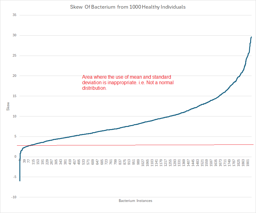
Microbiome data distributions frequently display extreme skewness—often greater than 20. In such cases, computing mean and standard deviation is simply incorrect.  My friend “Perplexity” writes Mean and standard deviation become inappropriate measures for computing significance if the distribution’s skewness is substantial—specifically, when the absolute skewness exceeds ±2.

Removing the Skewness

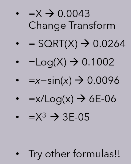
The simple answer comes from Perplexity and is below. My personal objective was not merely to reduce skew to be below 2, but as with all good operations research temperaments: optimization — i.e. reduce skew to be as close to 0 as possible!

For very skewed data, several transformation techniques are commonly used to reduce skewness and improve the suitability of data for statistical analysis. These methods alter the distribution to be closer to normal, helping stabilize variance and improve model fitting.​

Common Transformations for Skewed Data

Log Transformation: Taking the logarithm (often natural log) of each data point helps compress large values and is especially effective for positively skewed (right-skewed) data. Note that data must be strictly positive for log transformation to work.​

Square Root Transformation: The square root function less aggressively compresses data than log and works for moderately skewed data. It can be applied if all values are non-negative.​

Box-Cox Transformation: This is a flexible power transformation where a parameter (λ) is fit to minimize skew. Box-Cox works only on data that is strictly positive, but can substantially reduce skewness.​

Yeo-Johnson Transformation: An extension of Box-Cox, this method operates on data that includes zeros or negative values. It’s suitable for both positive and negative skewness.​

Quantile Transformation: Maps data to a specified distribution (often normal), distributing the values more evenly. It’s a non-linear method and often used when other transformations fail to sufficiently normalize skewed data.​

Power Transformations (Squared/Cubed): For negatively skewed (left-skewed) data, raising values to a higher power (e.g., squared, cubed) can help normalize the distribution.​

Inverse/Retransformation: For extreme cases, using the reciprocal (inverse) of the data can sometimes reduce skewness, but interpretation becomes less intuitive.​

Selecting the Right Transformation

The nature of the skew (positive or negative), the presence of zeros or negatives, and the degree of skewness guide the selection. Always visualize and evaluate the distribution after transformation to ensure that the resulting data meets the needs of your analysis.

Criteria for Selecting the Transformation

My approach is to objectively identify the optimal transformation supported by quantitative evidence rather than relying on subjective visual appeal. Because bacteria influence each other, we expect that a good transformation will maximize the coefficient of determination (R-squared, R2) across all bacterial pairs. R2 measures how well a regression model explains the variation in a dependent variable using independent variables. So in addition to reducing skew to near zero, we also want to optimize R-squared. The R-square is very significant for creating Markovian Matrices that may allow treatment progression to be modelled.

For the reference dataset, we include all bacterial pairs that have at least 25 counts, following recommendations from A solution to minimum sample size for regressions (2020).

Example: The reference set of 1000 shotgun samples has a total of 957,193 different sample id x taxon pairs.

• 13,083 different taxons
• 4,975,346 pairs that meet this criteria

To make your life easier, this is the query to get the pairs to be evaluated in T-SQL

SELECT A.taxon,B.Taxon
FROM [Reference_10M] A
JOIN [Reference_10M] B
ON A.Id=B.Id and A.Taxon <> B.Taxon
Group By A.Taxon,B.Taxon
Having count(1) >=25

Next, we need to calculate the R2 values across different data transformations to determine which yields the best performance. This process can benefit from competition among several graduate students, each striving to discover the optimal transformation. I was pleased when my colleague, Valentina Goretzki, identified a transformation that surpassed my own candidate solution. For more background, see my earlier post on methodology for the R² public site.

Compare these to the performance of my original preferred method: R² =0.23. The transformation will be unique to the processing of the microbiome data and likely be deemed proprietary and a trade secret. This is well stated by Scott Jackson below, and I have seen it with different reference sets from different labs.

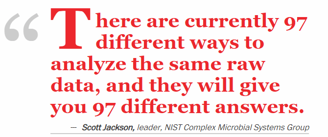
From The taxonomy nightmare before Christmas…

Be prepared to burn computer time!

To do a first run of the 8 methods cited above means doing 50 million coefficient of determination computation initially. Then comparing which is superior (i.e. create a 8×8 matrix showing the better counts for each combination).

Of course, we want to improve the transformations until you are at least close to the numbers showing on the Microbiome Taxa R² Site for the lab data that is in your reference set. Ideally better (since thanks to Valentina Goretzki we have superior internal numbers)!

The Big Win — Significance for Symptoms and Conditions

If you look at the Modelled Probiotics based on self-declared symptoms page that uses our earlier transformation and a similar transformation applied to data from Biomesight (a provider of 16s microbiome tests) you will see P < 0.0001 being available. The highest z-score was -103.9. Instead of reporting a couple of significant bacteria in studies, you may have dozens.

Z-Score	Instances
3	37,033
4	14,236
5	4,685
6	1,422
7	455
8	164
9	43
10	24

I am by training a Operation Research person and that means developing and using models, frequently complex models. I believe the above effort will result in massive payoffs.

Standard Error of Means

For one significant bacteria, I compared the z-score from taking the percentage against the transformation and got the following results for one symptom-bacteria pair:

• Percentage: 2.86
• Transformation: 9.09

For a different symptom-bacteria pair, we got the scores below

• Percentage: 1.36 or P < 0.09
• Transformation: 3.00 or P < 0.0013

One is far superior for detecting associations.

Machine Learning

When I began working on microbiome analysis, I initially employed machine learning techniques—reflecting the standard approach at Amazon, where I was employed at the time. However, I found the outcomes disappointing and not as robust as anticipated. My subsequent experiments highlighted a key limitation of methods based primarily on logistic transformations.

For illustration, I ran several analyses on Biomesight data for a given symptom, using both the original percentage values and various transformations. The dataset included over 2,200 bacterial taxa across more than 4,200 unique samples. The results, summarized in the table below, were generated using the Stochastic Dual Coordinate Ascent (SDCA) optimization algorithm, which applies a logistic model to the data. There is not much difference seen.

Note: This was done using not reported as zeroes.

	Area Under the Curve	F1 Score	Accuracy
Above or Below Average (Binary)	62.12%	16.30%	82.75%
Above or Below Transformed Average (Binary)	62.10%	16.39%	82.87%
Percentage	62.09%	16.57%	83.09%
Transformed Percentage	62.08%	16.30%	82.75%
Transformed Category	62.12%	16.48%	82.98%
Transformed Percentage with alternative handling of missing data.	62.11%	16.57%	83.09%
Above or below average of above	62.11%	16.76%	83.31%

The use of the logistic model transformation on top of raw data and transformed data effectively mask the differences [“the great equalizer”]. The great contrast that we saw with the z-score above is lost.

Accuracy

Accuracy is the simplest metric. It indicates the proportion of total correct predictions (both positive and negative) out of all predictions made. For example, if 90 out of 100 predictions are correct, the accuracy is 90%.
Accuracy works well when the classes are balanced, but can be misleading if one class dominates (class imbalance).

F1 Score

The F1 Score is the harmonic mean of Precision and Recall, combining them into a single value that balances both.

• Precision measures how many of the predicted positive cases were actually positive (focuses on false positives).
• Recall measures how many actual positive cases were correctly identified (focuses on false negatives).
  F1 Score is especially valuable when you have imbalanced classes and want a balance between precision and recall. An F1 score of 1 means perfect precision and recall, while 0 means very poor performance.

AUC (Area Under the Curve)

AUC usually refers to the area under the ROC curve (Receiver Operating Characteristic curve). It measures the model’s ability to distinguish between classes across all classification thresholds.

• An AUC of 1 means perfect separation of positive and negative classes.
• An AUC of 0.5 means the model performs no better than random chance.
  AUC is useful when you care about the model’s ranking ability and behavior at different decision thresholds rather than just accuracy.

Applying to an Individual’s Microbiome

Consider two scenarios:

• The individual has a diagnosis or symptom you’ve already modeled with regression:
  • Flag bacterial taxa whose levels exhibit statistically significant shifts relative to the model.
  • From those taxa, infer the most probable interventions to normalize the shifts (see below).
• There is no direct match or insufficient information:
  • Use the profile to predict potential diagnoses or risk patterns.
  • Propose early, person-specific interventions (e.g., diet adjustments) to steer the microbiome toward a healthier state.

Two Models for Prediction

The following are two thumbnails of methods which has had promising results:

• Linear and Mixed Linear Programming Models
• Probability Density Models

My own algorithms have had very good success, often 80-100% correct prediction of the top 10 symptoms from a new sample when reviewed by the client.

Using Linear and Mixed Linear Programming Models

Regression can be done using linear programming or integer programming models, although it is not the most conventional approach compared to classical regression methods. It is my preferred approach, libraries like Google OR-Tools are available.

• Linear programming can be applied to regression tasks through optimization formulations, where the goal is to minimize an objective function such as the sum of absolute deviations (L1 regression) or other loss functions. This approach can handle linear regression problems by framing coefficient estimation as a linear optimization problem.
• Integer programming can be used in regression contexts where you want to impose discrete constraints on variables, for example, to select variables (feature selection), enforce sparsity, or manage categorical variable encoding directly within the regression framework.
• These optimization-based regressions are especially useful when classical least squares regression assumptions are violated or when additional complex constraints are needed.
• For categorical variables, the encoding (like dummy variables) can be incorporated as part of the optimization model through integer variables that represent category memberships or selections.

Thus, linear and integer programming methods provide a flexible, optimization-centric framework for regression and forecasting, allowing incorporation of categorical variables and customized constraints beyond traditional statistical regression techniques. However, these are typically used in more advanced or specific applications rather than standard regression analysis.

Example, k is the sample number, c(k,n) is the amount of bacteria n,

Y(k)=c(k,1)⋅x1+c(k,2)⋅x2+…+c(k,N)⋅xN  or Y(k)=∑_i=1^Nc(k,i)⋅x_i.

With the goal of minimizing (or maximizing):  ∑_kY(k).

Probability Density Models

This approach crystallized after reviewing several odds charts like the one below. The signal isn’t a simple “high vs. low” level; rather, risk appears when a bacterium’s abundance falls within specific “risk zones.” The pattern reminded me of electron probability density clouds in atoms. Why does this occur? Likely due to quorum sensing and the extensive network of microbial interactions.

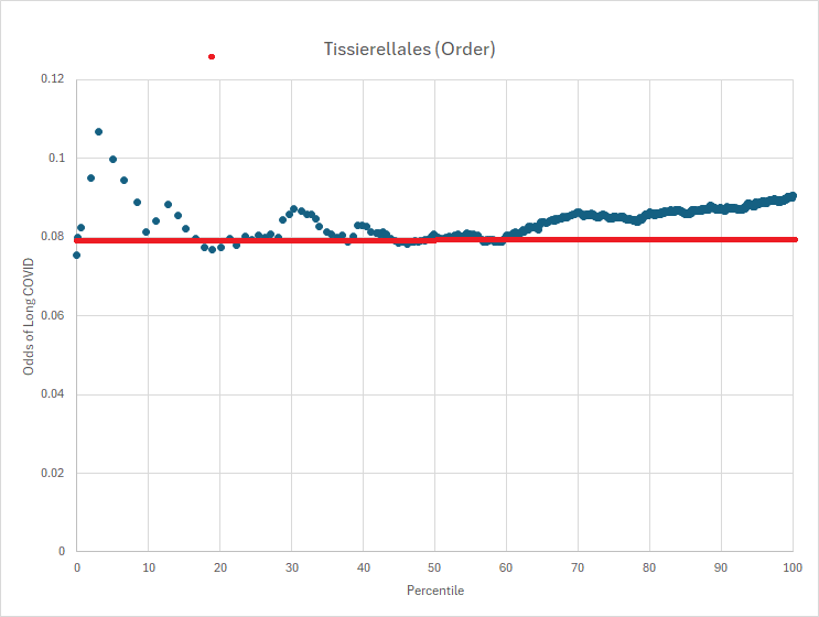
The forecasting algorithm is to apply these odds density function to the sample to estimate various diagnosis or symptoms.

Fixing the Microbiome

This depends very much on whether your database of modifiers is dense or very very sparse. Using a microbiome model I am able to get a high density database for probiotics because of the R2 above, I can estimate the likely impact of one bacteria(i.e. probiotic) on another bacteria. A sample results is shown below:

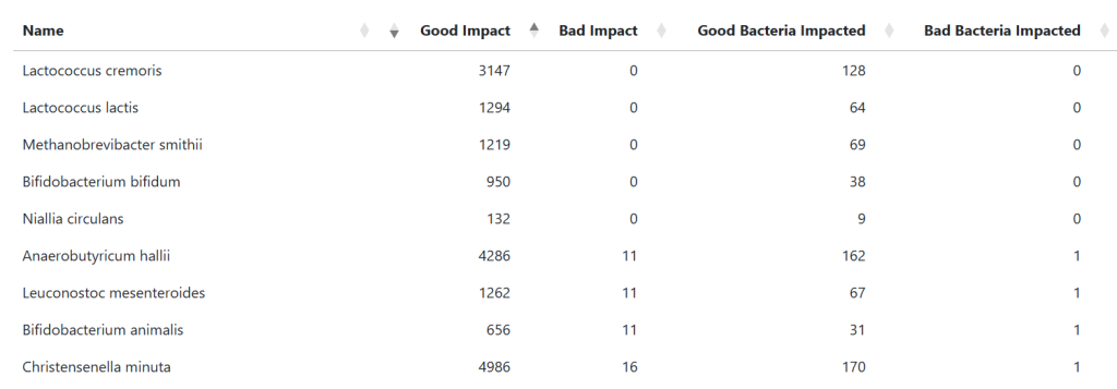
There are usually a small number of items that “does no harm” and then we enter the mixed scenario and occasionally the “do only harm”. I prefer to do lowest risk (no harm) suggestions.

When we move to sparse data, i.e. gluten-free diet, Mediterranean diet, barley, rye, wheat, etc. We will often find there is not a single PubMed study on the bacteria that has been shifted. There are a variety of approaches possible — for example, looking at what increases the probiotic bacteria identified above, or doing extrapolations to other members of the taxonomy hierarchy.

No Data identification of Bacterium to Modify

In this scenario, we have a microbiome with no additional information. There are two common approaches:

• Using an aggregation of the bacteria reported significant in any study reported on pub med
  • For those reported high or low, flag the bacteria if the sample is in the top or bottom 5-10% of samples appropriately (or one of the methods below). This gives us a target set of bacteria.
• Deriving reference ranges for some collection of bacteria. Some options for determining reference ranges for data with substantial skew:
  • Percentile (Non-parametric) Method:
    Calculate reference intervals using percentiles (e.g., the 2.5th and 97.5th for a two-sided range). This method does not assume normality and is robust to skew. CLSI guidelines recommend a minimum of 120 samples and calculating confidence intervals using resampling or rank-based techniques.
  • Data Transformation:
    Apply transformations such as logarithmic or Box-Cox to reduce skewness and then use parametric methods for reference range estimation. The transformed data is analyzed as if approximately normal, and limits are back-transformed for interpretation. The choice of transformation depends on the degree and direction of skew (Box-Cox λ parameter: log-normal for right-skew, square-root for moderate skew).
  • Robust Methods:
    Use approaches like the robust method (e.g., median and MAD—Median Absolute Deviation), which iteratively downweights extreme values and calculates reference limits based on weighted estimates. This method is suitable for moderate sample sizes and strong skew.
  • Indirect Statistical Algorithms:
    Algorithms such as refineR or kosmic separate non-pathological and pathological distributions in large observational datasets and are especially useful when direct reference populations are hard to obtain or data is heavily skewed.
  • Parametric Modeling:
    Fit distributions capable of representing skew (like log-normal or skew-normal) or use regression-based approaches modeling mean, variance, and skewness, as described by Royston and Wright, with age or other covariates included as needed.

The key difference is the amount of “noise”, i.e. false identification of insignificant bacteria.

Summary

This gives a high level overview of issues encountered with doing microbiome analysis and using a microbiome to generate suggestions to improve an individual’s microbiome.

Special thanks to my 1972 probability (not statistics) instructor, Cindy Greenwood, Professor Emerita at the University of British Columbia. She had a special interest in plague modelling then and introduced me to dozens of probability models and Markovian Processes in the days when we still did statistics and probability using pen and paper. This was the same year that  the world’s first scientific handheld calculator, HP-35, capable of performing logarithmic and trigonometric functions in addition to basic arithmetic was released at a cost of several months salaries.